Plotting Mathematical Functions in Ruby, Inside Jupyter

March 13, 2026

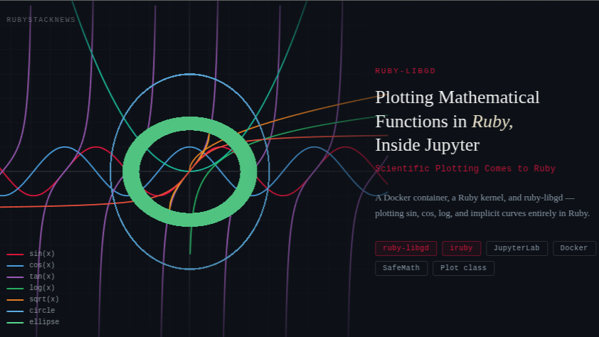
ruby-libgd: Scientific Plotting Comes to Ruby

The Envy We Never Talked About

Anyone who has spent serious time with Ruby and then watched a Python developer type plt.show() to produce a beautiful Matplotlib graph in a Jupyter notebook knows the feeling. It is not quite jealousy — Ruby is still the most expressive language most of us have ever touched — but it is a quiet recognition that Python had something we did not.

I came to Ruby after years in PHP, C, and C++. I dedicated myself to mastering it, and I never regretted that decision. Ruby’s syntax turns ideas into algorithms with a naturalness that no other language I know has matched. But scientific visualization? That was always Python’s unfair advantage.

Today, on a Friday afternoon, I want to share something that closes that gap: a Docker container running JupyterLab with a full Ruby kernel, backed by ruby-libgd, plotting Sin, Cos, Log, and arbitrary mathematical functions entirely in Ruby. No Python. No wrappers. Just Ruby.

Building the Container

The foundation is a Docker image that installs the Ruby kernel for Jupyter alongside the system libraries that ruby-libgd needs. Here is the complete Dockerfile:

FROM python:3.11
RUN apt-get update && apt-get install -y \
    ruby-full \
    build-essential \
    libgd-dev \
    libgd3 \
    libgd-tools \
    valgrind \
    libzmq3-dev
RUN printf "prefix=/usr\n\
exec_prefix=\${prefix}\n\
libdir=\${exec_prefix}/lib/x86_64-linux-gnu\n\
includedir=\${prefix}/include\n\
\n\
Name: gd\n\
Description: GD Graphics Library\n\
Version: 2.3\n\
Libs: -L\${libdir} -lgd\n\
Cflags: -I\${includedir}\n" \
> /usr/lib/x86_64-linux-gnu/pkgconfig/gd.pc
RUN pip install jupyterlab
RUN gem install iruby
RUN iruby register --force
RUN gem install ruby-libgd
RUN gem install libgd-gis
EXPOSE 8888
CMD ["jupyter", "lab", "--ip=0.0.0.0", "--port=8888", "--no-browser", "--allow-root", "--ServerApp.token="]What Each Layer Does

The image is built on top of python:3.11 — not because we need Python for plotting, but because JupyterLab is a Python application. The Ruby kernel runs as a plugin inside it.

• ruby-full ruby-full — installs the complete Ruby runtime and gem toolchain.
• libgd-dev libgd-dev / libgd3 — the C library that powers ruby-libgd’s pixel drawing engine.
• libzmq3-dev libzmq3-dev — ZeroMQ is the message transport that connects the Ruby kernel to the browser frontend.
• iruby iruby — the Ruby kernel for Jupyter. After installing, iruby register –force registers it so JupyterLab can discover it.
• gd.pc The pkg-config file — libgd ships without one on Debian, so the RUN printf block writes it manually. Without this, gem install ruby-libgd cannot locate the library headers.

The pkg-config Fix

This is the most non-obvious step in the whole setup. When ruby-libgd compiles its native extension it calls pkg-config –libs gd to find where libgd is installed. On Ubuntu and Debian, libgd-dev does not ship a .pc file, so pkg-config returns nothing and the build fails.

The printf block in the Dockerfile writes the file directly into the system pkg-config path. It tells the build system exactly where the library and headers live, and the gem compiles cleanly.

If you are on an ARM machine (Apple Silicon, AWS Gravitium) replace x86_64-linux-gnu with aarch64-linux-gnu in the libdir path.

Running the Container

Build the image once, then mount your working directory and run:

docker build -t ruby-jupyter .
docker run -it -p 8888:8888 -v $(pwd):/work ruby-jupyter

Open http://localhost:8888 in your browser. Create a new notebook and select the Ruby kernel from the kernel picker. You are ready to plot.

The SafeMath Evaluator

Before looking at the Plot class, it is worth understanding the expression evaluator underneath it. Earlier versions of this code used Dentaku — a formula evaluator designed for business logic. Dentaku works, but it has significant gaps for scientific use: trigonometric functions operate in degrees instead of radians, natural logarithm is not available, and inverse trig functions are missing entirely.

The replacement is SafeMath — a thin module that evaluates expressions inside an isolated context class that includes Ruby’s own Math module:

module SafeMath
  class EvalContext
    include Math
    def pi; Math::PI; end
    def e;  Math::E;  end
    def initialize(vars)
      vars.each do |k, v|
        val = v.to_f
        define_singleton_method(k) { val }
      end
    end
    def ln(v);    Math.log(v);   end   # natural log
    def log(v);   Math.log(v);   end   # alias
    def log10(v); Math.log10(v); end
    def log2(v);  Math.log2(v);  end
    def abs(v);   v.abs;         end
    def cbrt(v);  Math.cbrt(v);  end
    def eval_expr(expr)
      result = eval(expr)
      return nil unless result.is_a?(Numeric)
      return nil if result.infinite? || result.nan?
      result.to_f
    end
  end
  def self.evaluate(expr, vars = {})
    EvalContext.new(vars).eval_expr(expr)
  rescue Math::DomainError, ZeroDivisionError
    nil
  end
end

Variables like x and y are injected as singleton methods on the context object, so the eval call sees them as local identifiers. Domain errors — log of a negative number, sqrt of a negative — return nil, and the drawing code skips that sample cleanly.

The full function support available in every expression:

• Trigonometric (radians): sin, cos, tan, asin, acos, atan
• Hyperbolic: sinh, cosh, tanh
• Logarithmic: log / ln (natural), log10, log2
• Algebraic: sqrt, cbrt, abs, exp
• Rounding: floor, ceil, round
• Constants: pi, e

The Plot Class

The Plot class wraps ruby-libgd’s GD::Image into an API that feels natural to write in a Jupyter cell. The complete class definition goes in one cell at the top of the notebook. Every subsequent cell just calls it.

Constructor

plot = Plot.new(
  width:  600,
  height: 600,
  xmin:  -10.0,
  xmax:   10.0,
  ymin:  -10.0,
  ymax:   10.0
)

All parameters are optional. The defaults give a 600×600 canvas spanning −10 to 10 on both axes.

Adding Curves

Every curve is added with a single method call. The type keyword selects the rendering algorithm:

# Explicit: y = f(x)
plot.add("sin(x)")
plot.add("cos(x)",  color: GD::Color.rgb(60, 130, 220))
plot.add("tan(x)",  steps: 6000)   # more samples around asymptotes
plot.add("log(x)")
plot.add("sqrt(x)")
plot.add("exp(x) / 500.0")
plot.add("x**2 / 10.0")
plot.add("(x + 56)**3 / 50000.0")
# Implicit: f(x, y) = 0
plot.add("x**2 + y**2 - 9",   type: :implicit)             # circle r=3
plot.add("(x-2)**2 + y**2 - 4", type: :implicit)           # circle centered at (2,0)
plot.add("x**2/9.0 + y**2/4.0 - 1", type: :implicit)      # ellipse

Colors are allocated via GD::Color.rgb(r, g, b) and passed directly to drawing methods — this is how ruby-libgd’s API works. If you omit the color option, Plot cycles through a built-in 12-color palette automatically.

Rendering

plot.render("/work/graph.png")

render saves the file and calls Jupyter’s render() helper to display the image inline. The path /work maps to the directory you mounted with -v $(pwd):/work, so the file is also available on your host machine immediately.

How the Two Rendering Strategies Work

Explicit curves — tracing

For functions where y is directly computable from x, the algorithm sweeps x from xmin to xmax in small steps, evaluates y = f(x) at each point, converts to pixel coordinates, and connects consecutive points with line segments.

The discontinuity guard detects vertical jumps larger than one third of the image height and resets the previous point. This is what makes tan render correctly — instead of drawing a vertical line across an asymptote, it simply lifts the pen.

steps.times do |i|
  x = xmin + (i.to_f / steps) * (xmax - xmin)
  y = SafeMath.evaluate(expr, x: x)
  next unless y                           # domain error — skip
  px, py = to_px(x, y)
  next unless in_bounds?(px, py)          # off canvas — reset
  if prev && (py - prev[1]).abs > height / 3
    prev = nil                            # discontinuity — lift pen
  end
  img.line(prev[0], prev[1], px, py, color) if prev
  prev = [px, py]
end

Implicit curves — pixel sampling

For equations involving both x and y — circles, ellipses, and algebraic curves where y cannot be isolated — the algorithm tests every pixel. It maps pixel coordinates back to world coordinates, evaluates f(x, y), and colors the pixel if the absolute value is below a threshold.

The threshold controls perceived line thickness. A value of 0.30 is a good starting point. Reduce it for tighter lines on small curves, raise it for larger ones that might otherwise appear dotted.

width.times do |px|
  height.times do |py|
    x   = xmin + (px.to_f / width)  * (xmax - xmin)
    y   = ymax - (py.to_f / height) * (ymax - ymin)
    val = SafeMath.evaluate(expr, x: x, y: y)
    img.set_pixel(px, py, color) if val && val.abs < threshold
  end
end

Example Notebooks

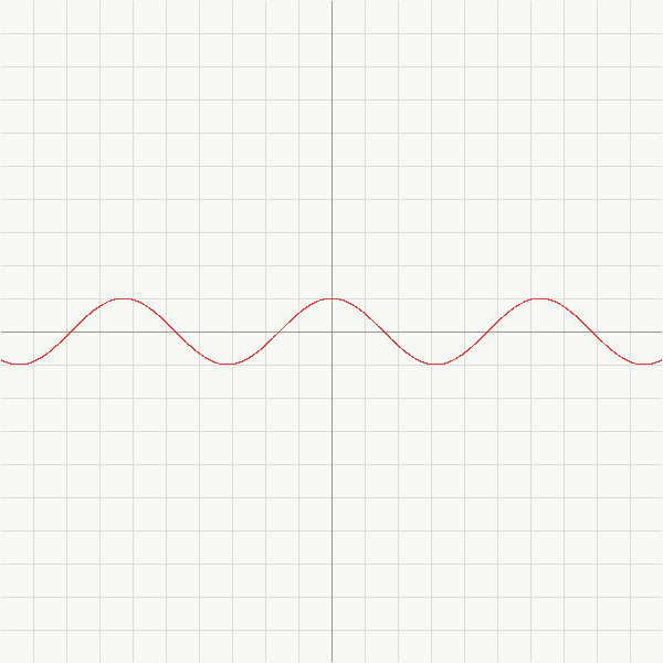
Notebook 1 — Classic trigonometric functions

require 'gd'
# ... SafeMath and Plot class defined above ...
plot = Plot.new
plot.add("sin(x)")
plot.add("cos(x)")
plot.add("tan(x)", steps: 6000)
plot.render("/work/trig.png")

Notebook 2 — Logarithms and roots

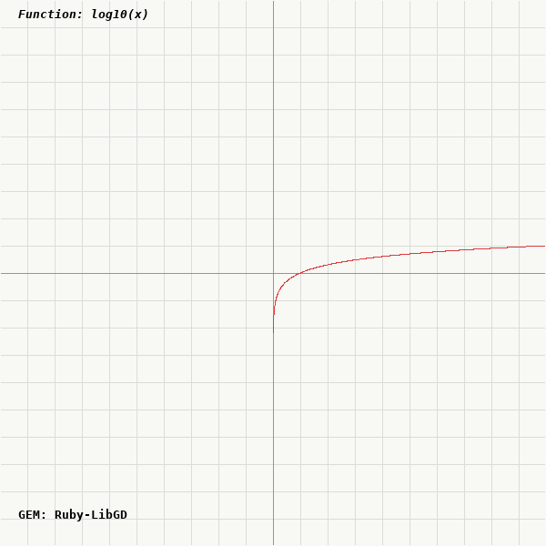
plot = Plot.new(xmin: 0.01, xmax: 10, ymin: -4, ymax: 4)
plot.add("log(x)")
plot.add("log10(x)")
plot.add("log2(x)")
plot.add("sqrt(x)")
plot.add("cbrt(x)")
plot.render("/work/logs.png")

Notebook 3 — Polynomial with large coefficients

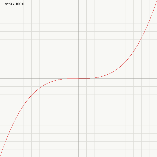
One of the first expressions I tested when the notebook came to life was (x + 56)^3. Scaling it to fit the viewport is just arithmetic — divide by a constant until the curve sits comfortably within the window.

plot = Plot.new(xmin: -60, xmax: -50, ymin: -200, ymax: 200)
plot.add("(x + 56)**3 / 1000.0")
plot.render("/work/cubic.png")

Notebook 4 — Implicit curves: circles and ellipses

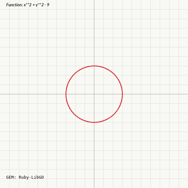
plot = Plot.new
plot.add("x**2 + y**2 - 9",            type: :implicit)
plot.add("x**2 + y**2 - 49",           type: :implicit, threshold: 0.45)
plot.add("x**2/16.0 + y**2/4.0 - 1",  type: :implicit)
plot.add("(x-3)**2 + (y-3)**2 - 4",   type: :implicit)
plot.render("/work/circles.png")

What Is Coming Next

The Plot class you see here will be refactored into a standalone gem — a clean plotting interface that sits on top of ruby-libgd. The goal is an API where you can produce a publication-quality graph from a single require and three lines of code.

The immediate roadmap:

• Axis labels and tick marks rendered with TrueType text via ruby-libgd’s text method.
• A legend panel mapping curve colors to expression strings automatically.
• A plot.show method that detects the Jupyter context and inlines the image without an explicit path.
• Parametric curve support — add_parametric(x_expr, y_expr, t_range: 0..Math::PI*2).
• PNG and JPEG output with format auto-detection from the file extension.

Closing Thoughts

Watching sin(x) appear in a Ruby Jupyter notebook for the first time felt a little like vindication. Ruby has always deserved this. The language that made web development joyful, that turned configuration into code and DSLs into art, now has a path to the same exploratory data visualization that made Python so dominant in scientific communities.

ruby-libgd is the foundation. The notebooks are the proof. The gem is coming.

If you want to follow along, star the repository, try the Docker setup, and let me know what functions you plot first.