Ruby for Data Science — Is It Possible? – Linking Ruby knowledge from the most remote places in the world.

March 16, 2026

Published on RubyStackNews

After the last article, Jupyter proved to be an awesome sandbox for testing code interactively. I spent the entire weekend asking myself one question: can Ruby render a real 3D plot? I started convinced the answer was no. By Sunday night, ruby-libgd had proven me wrong.

The question nobody asks

When developers think about data science, they think Python. They think NumPy, pandas, matplotlib. Ruby almost never enters the conversation — and honestly, for years that was fair. Ruby had no serious image generation story. No plotting library worth mentioning. The ecosystem simply wasn’t there.

But things changed quietly. ruby-libgd brings native GD library bindings to modern Ruby, and with it a real 2D raster engine: pixel operations, line drawing, polygon fills, alpha blending — everything you need to build a renderer from scratch.

So the question became: how far can you push it?

Starting with 2D — the Plot class

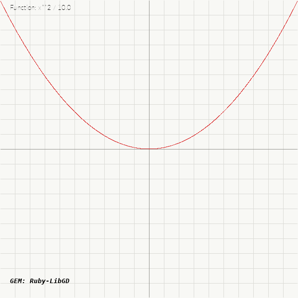
Before tackling 3D, I built a 2D function plotter using ruby-libgd and Ruby’s own Math module. No external formula evaluators. No dependencies beyond the gem itself.

ruby

			
require 'gd'
plot = Plot.new(xmin: -10, xmax: 10, ymin: -10, ymax: 10)
plot.add("sin(x)")
plot.add("cos(x)")
plot.add("log(x)")
plot.add("x**2 + y**2 - 25", type: :implicit)
plot.render("/work/graph.png")

		

Two rendering strategies in one class:

Explicit curves (y = f(x)) — traced by sampling x values and connecting points with lines. Discontinuity detection handles functions like tan(x) that jump at asymptotes.
Implicit curves (f(x,y) = 0) — pixel sampling. Every pixel is evaluated and painted if the expression is close enough to zero. This handles circles, ellipses, and any curve where y can’t be isolated.

The evaluator runs expressions inside an EvalContext that includes Ruby’s Math module, so sin, cos, log, sqrt, exp, atan — everything works natively, in radians.

Going 3D — the impossible part

This is where it got interesting.

3D graphics on a 2D raster image means implementing the entire pipeline in pure Ruby:

1. Rotation — two rotation matrices, yaw and pitch, let you orbit the scene by changing two angles.

ruby

			
# Yaw — rotate around Z axis
x1 =  x * cos_y + y * sin_y
y1 = -x * sin_y + y * cos_y
# Pitch — rotate around X axis
y2 = y1 * cos_p - z * sin_p
z2 = y1 * sin_p + z * cos_p

		

2. Perspective projection — divide by depth. Objects further from the camera appear smaller.

ruby

			
def project2d(x, y, z)
  denom = (cam_dist - z).abs
  sx = (fov * x / denom + width  / 2.0).to_i
  sy = (-fov * y / denom + height / 2.0).to_i

[sx, sy]

end

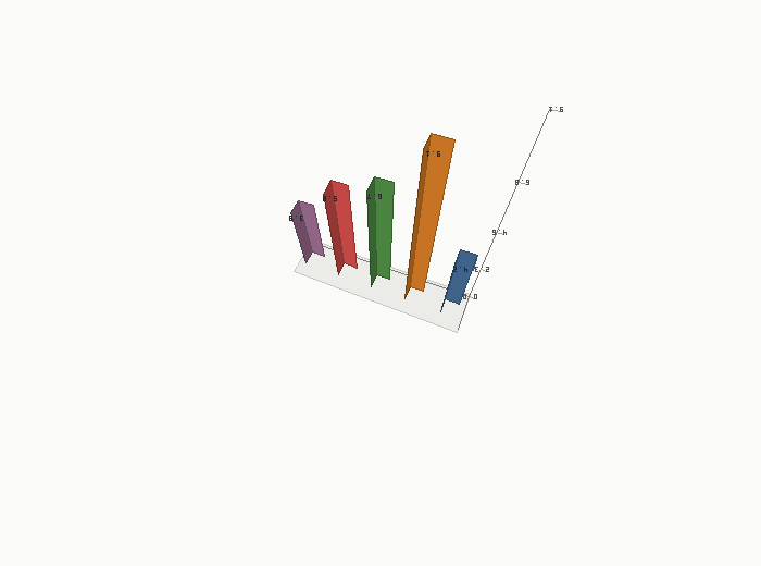
3. Painter’s algorithm — sort all patches back-to-front by their average camera depth, then draw them in that order. No Z-buffer. No GPU. Just Array#sort_by.

ruby

			
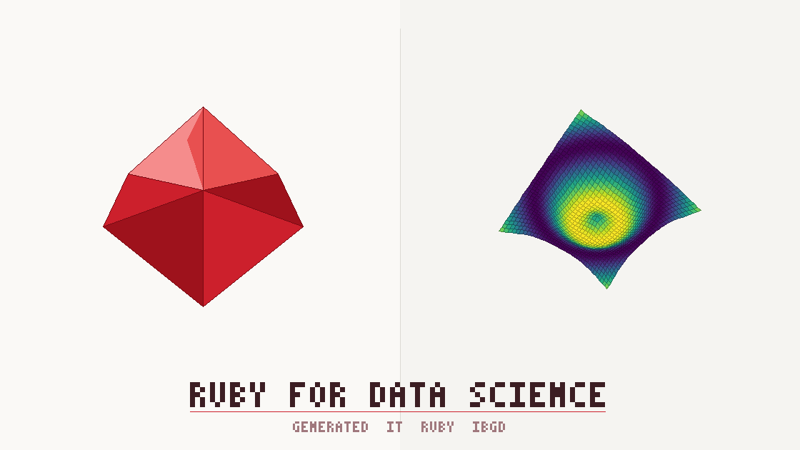
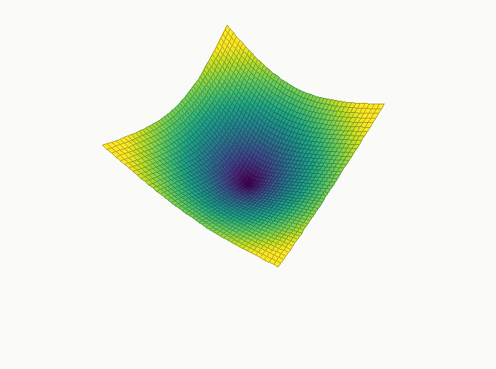
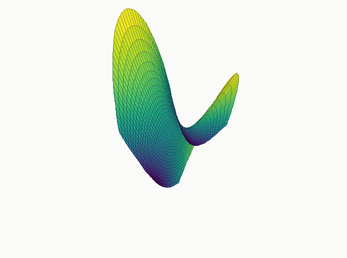
patches.sort_by! { |p| -p[:depth] }
patches.each { |p| draw_filled_polygon(img, p[:pts2d], color) }

4. Colormap — z-value mapped through 11 viridis stops via linear interpolation. The lowest z is deep purple, the peak is bright yellow — immediately recognizable to anyone who has used matplotlib or seaborn.

The results

The API ended up clean enough that each plot is a single chain:

ruby

			
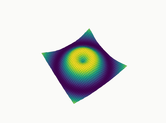
# Ripple surface — z = sin(sqrt(x² + y²))
Plot3D.new(resolution: 50, yaw: 35, pitch: 28)
  .surface("sin(sqrt(x**2 + y**2))")
  .render("/work/ripple.png")
# Saddle surface — z = x² - y²
Plot3D.new(yaw: 40, pitch: 25, xmin: -3, xmax: 3, ymin: -3, ymax: 3)
  .surface("x**2 - y**2")
  .render("/work/saddle.png")
# Wave surface — z = cos(x) * sin(y)
Plot3D.new(yaw: 30, pitch: 30, xmin: -4, xmax: 4, ymin: -4, ymax: 4)
  .surface("cos(x) * sin(y)")
  .render("/work/wave.png")
# Paraboloid — z = x² + y²
Plot3D.new(yaw: 35, pitch: 28, xmin: -3, xmax: 3, ymin: -3, ymax: 3)
  .surface("x**2 + y**2")
  .render("/work/paraboloid.png")

		

(Images below — generated entirely in Ruby, rendered in Jupyter)

What Jupyter adds

Running this inside IRuby/Jupyter changes the workflow completely. You tweak yaw: 35 to yaw: 45, re-run the cell, see the result inline. It’s the same iterative loop that made Python notebooks popular for data exploration — and it works just as well for Ruby.

The Plot3D class is defined once at the top of the notebook. Every cell below it is just configuration and a .render() call. No server restarts. No constant redefinition warnings. No state leaking between runs.

The honest verdict

Can Ruby do data science? Not yet — not fully.

What’s missing compared to a mature Python stack: statistical computation (no NumPy equivalent), dataframe support (though rover is promising), and a complete plotting library with axes, legends, and annotations built in.

What’s here right now: a solid image engine, a working 3D renderer built in a weekend, and a Jupyter workflow that feels natural for exploratory work.

Languages do not evolve on their own. They evolve because developers get curious, spend a weekend on something that probably won’t work, and then share what they find.

Ruby has always grown that way — from web frameworks nobody believed in, to testing tools that changed how the whole industry writes code. Data visualization is just the next boundary worth pushing.

This is one experiment. What the community builds on top of it is the interesting part.